Exporting reports

DAGassist reports are meant to leave your R console: as an appendix table in a paper, a response to a reviewer, or a file for a co-author. Users can easily export reports through two arguments. type sets the format, and out sets the file path and name. This article explains how to export your DAGassist report. The examples use the voter-turnout data from the homepage.

library(DAGassist)

Formats at a glance

type	Produces	out	Also needs
"console" (default)	The report, printed in the console	Not used
"latex"	A LaTeX fragment to \input{} into a paper	Optional; prints the fragment if omitted	modelsummary
"word" or "docx"	A Word document	Required	modelsummary, knitr, rmarkdown, and pandoc 2.0+
"excel" or "xlsx"	An Excel workbook, one sheet per section	Required	modelsummary
"text" or "txt"	A plain-text file with Markdown tables	Optional; prints if omitted	modelsummary, knitr
"dotwhisker" or "dwplot"	A dot-and-whisker plot (PNG)	Optional; displays the plot if omitted

The packages in the last column are suggested dependencies for each export format, so install them prior to exporting. RStudio ships with pandoc, so Word export works there without extra setup.

Generating individual and multiple reports

To produce every format at once, create a loop where each export is the same DAGassist() call with a different type and out:

out_dir <- tempdir()
formats <- c(latex      = "report.tex",
             word       = "report.docx",
             excel      = "report.xlsx",
             text       = "report.txt",
             dotwhisker = "report.png")

for (fmt in names(formats)) {
  DAGassist(turnout_dag,
            lm(turnout ~ income + state + age + polint + industry + elect_comp,
               data = turnout_data),
            type = fmt,
            out  = file.path(out_dir, formats[[fmt]]))
}

file.exists(file.path(out_dir, formats))
#> [1] TRUE TRUE TRUE TRUE TRUE

To write a single file, drop the loop:

DAGassist(turnout_dag,
          lm(turnout ~ income + state + age + polint + industry + elect_comp,
             data = turnout_data),
          type = "latex",
          out  = "tables/dagassist.tex")

Choosing what goes in the report

The same arguments that specify the console output contents affect exported reports:

• show selects sections. show = "models" exports only the model comparison, whereas show = "roles" exports only the roles table.
• labels replaces variable names with readable labels. It takes a named character vector, or a data frame.
• estimand adds the total- and direct-effect columns described in Total and direct effects. Weight and balance diagnostics are exported alongside them.
• exclude adds canonical-set variants without neutral controls, as extra Canon. (-NCO) or Canon. (-NCT) columns.
• omit_intercept and omit_factors (both TRUE by default) hide the intercept and factor-level rows from the table. The terms still enter the regression.

For a publication table, set labels and show = "models":

turnout_labels <- c(
  income     = "Income",
  state      = "State",
  age        = "Age",
  polint     = "Political interest",
  industry   = "Industry",
  elect_comp = "Election competitiveness"
)

DAGassist(turnout_dag,
          lm(turnout ~ income + state + age + polint + industry + elect_comp,
             data = turnout_data),
          labels = turnout_labels,
          show = "models", type = "text", verbose = FALSE)

Term	Original	Minimal 1	Canonical
Income	0.281***	0.493***	0.492***
	(0.016)	(0.016)	(0.015)
State	0.331***	0.324***	0.332***
	(0.017)	(0.019)	(0.018)
Age	0.275***	0.273***	0.267***
	(0.017)	(0.020)	(0.019)
Political interest	0.420***
	(0.014)
Industry	-0.017		-0.010
	(0.015)		(0.016)
Election competitiveness	0.500***		0.506***
	(0.014)		(0.015)
Num.Obs.	5000	5000	5000
R2	0.596	0.423	0.525

• p-value legend: + < 0.1, * < 0.05, ** < 0.01, *** < 0.001.
• Controls (minimal): {age, state}.
• Controls (canonical): {age, elect_comp, industry, state}.

LaTeX

type = "latex" writes a fragment, not a full document, so you \input{} it where the table should appear. The tables use tabularray’s longtblr, so long tables break across pages. Add these lines to your preamble:

\usepackage{graphicx}   % rotated column headers in the roles table
\usepackage{tabularray}
\UseTblrLibrary{booktabs,siunitx}

The full report is labelled tab:dagassist, and a models-only table (show = "models") is labelled tab:dagassist-models, so you can refer to either with \ref{}.

Without out, the fragment is printed to the console, ready to paste into Overleaf:

DAGassist(turnout_dag,
          lm(turnout ~ income + state + age + polint + industry + elect_comp,
             data = turnout_data),
          labels = turnout_labels,
          show = "models", type = "latex")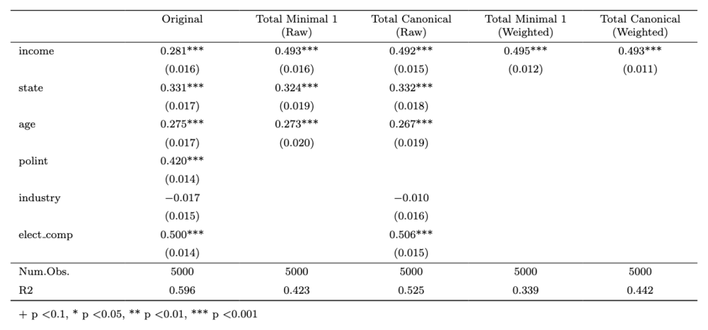

The model comparison table, typeset in LaTeX.

Word

type = "word" builds the report as Markdown and converts it to .docx with pandoc. To match a journal’s or your department’s styles, point DAGassist at a reference document once per session; pandoc copies its fonts, heading styles, and table styles:

options(DAGassist.ref_docx = "my-template.docx")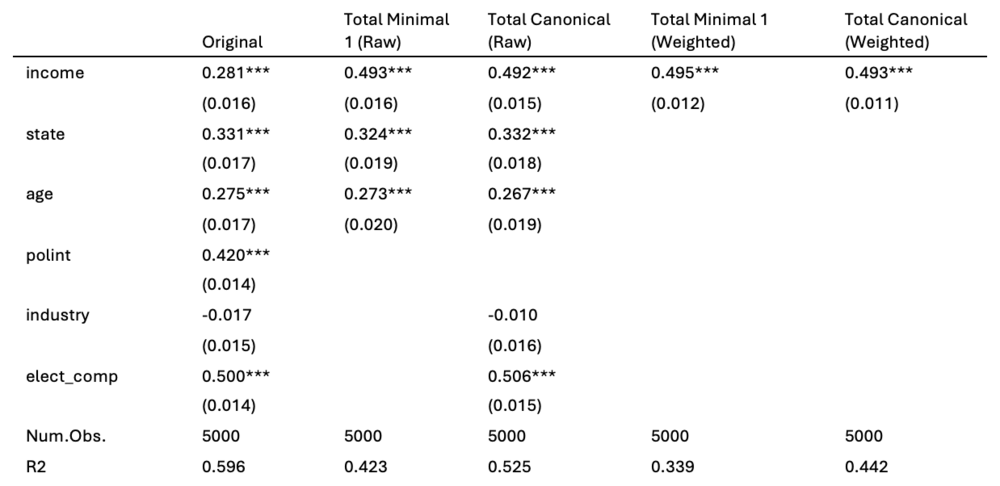

The report in a Word document.

Excel

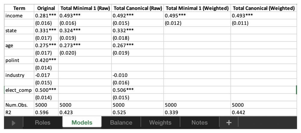
type = "excel" writes one sheet per section of the report, which makes the results easy to share with co-authors or reformat by hand:

readxl::excel_sheets(file.path(out_dir, "report.xlsx"))
#> [1] "Roles"   "Models"  "Balance" "Notes"

A Weights sheet is added when the report includes weighted estimates (estimand = "total" or "direct").

The Excel workbook.

Plain text and Markdown

type = "text" writes the report with Markdown tables. The file reads cleanly as plain text and renders as formatted tables on GitHub or in a reviewer response. Without out, it prints to the console; in an R Markdown or Quarto document, set the chunk option results = "asis" to render the tables, as this site does.

Dot-and-whisker plots

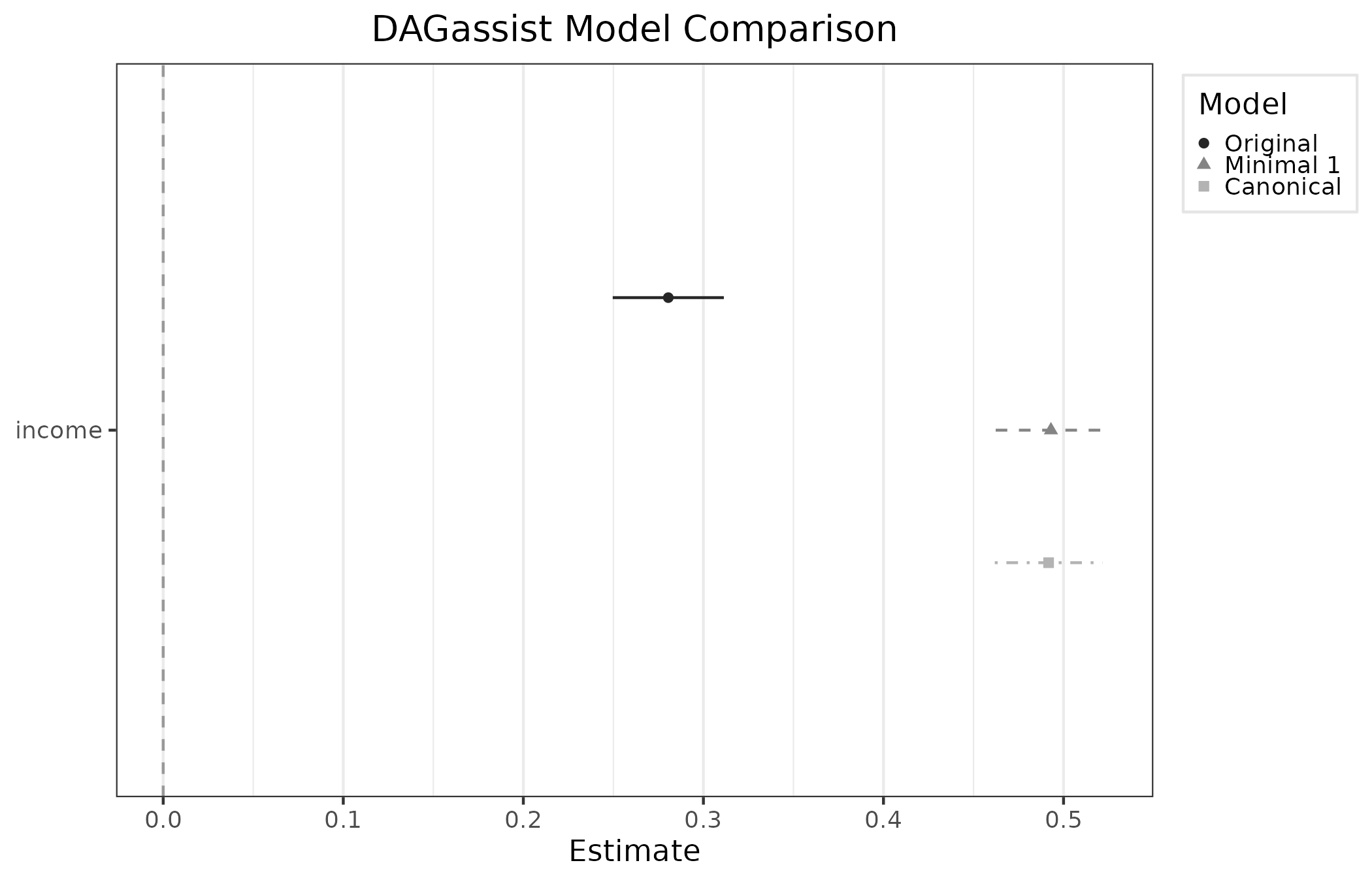
type = "dotwhisker" plots the exposure’s estimate and 95% confidence interval in each model. Without out, the plot is displayed; with out, it is saved as an 8 × 6 inch PNG at 300 dpi.

DAGassist(turnout_dag,
          lm(turnout ~ income + state + age + polint + industry + elect_comp,
             data = turnout_data),
          type = "dotwhisker")